Choosing a graph, and the line of best fit
What this lesson covers
- A distribution is formed from all the possible values of a variable and their frequencies. It can be shown using data visualisations that show patterns, trends, and variations and that include dot plots, bar graphs, frequency tables, box plots, histograms, time-series graphs, scatter plots, and two-way tables.
- A good data visualisation should allow viewers to discern the variable(s) and who the data was collected from, and then, depending on the type of visualisation, additional information such as frequency, proportions, patterns or trends, and units for numerical variables.
- In relationship investigations: sometimes one variable is thought of as predictive of the other variable; then the response or dependent variable is on the y-axis, and the ‘predictive’, explanatory, or independent variable is on the x-axis an eyeballed line or curve of best fit can be added for paired numerical data.
A graph is not decoration
- It is the picture of a distribution.
- So which graph you draw is decided by the data.
- Not by which one you find easiest to draw.
What a distribution actually is
- All the values your variable took.
- Together with how often each one happened.
- That pairing is the distribution. A graph shows it.
| Part | Detail | Note |
|---|---|---|
| All the values | that the variable took | |
| With their frequencies | how often each one happened | |
| Together | that is the distribution | |
| A graph | is a picture of it | not a decoration |
The kind of variable picks the graph
- One categorical variable: a bar graph.
- One numerical: a dot plot, a histogram, or a box plot.
- Two numerical and paired: a scatter plot.
| What you have | What to draw | Example |
|---|---|---|
| One categorical | bar graph | sport, year level |
| One numerical | dot plot, histogram, box plot | height, score |
| Two numerical, paired | scatter plot | hours against score |
| Numerical over time | time-series graph | rainfall by month |
| Two categorical | two-way table | sport by year level |
Why the wrong graph loses information
- Draw heights as a bar graph and each height becomes a category.
- You have thrown away the order, and the spacing.
- 150 is nearer 152 than 180, and a bar graph cannot say so.
| Choice | What happens | Note |
|---|---|---|
| Bar graph of heights | treats each height as a category | |
| What is lost | the order and the gaps | |
| Numbers have spacing | 150 is closer to 152 than to 180 | |
| A dot plot keeps it | so use that |
What a reader must be able to work out
- What was measured, and who it was measured on.
- The units, for anything numerical.
- A graph that needs you there to explain it has failed.
| Must show | Meaning | Where |
|---|---|---|
| The variable | what was measured | axis label |
| The group | who it was measured on | title |
| The units | for anything numerical | cm, minutes, dollars |
| The frequencies | or the pattern | depends on the graph |
And usually you draw more than one
- A dot plot shows every individual value.
- A box plot shows the quartiles from last lesson.
- Different graphs of the same data answer different questions.
Choosing a scale
- Data from 60 to 82 on an axis running to 1000 is a stripe.
- Run the axis from 60 to 85 and you can read it.
- Cover your data, with a little room. That is the whole rule.
| Data | Axis | Result |
|---|---|---|
| Data runs 60 to 82 | an axis of 0 to 1000 | everything in a stripe |
| Same data | an axis of 60 to 85, steps of 5 | readable |
| Rule of thumb | cover the data, with a little room |
Now the scale trick worth knowing about
- Two values: 100 and 105. A rise of five percent.
- Start the axis at zero and the bars look nearly identical.
- Start it at 95 and the second bar is twice the height.
| Version | What it looks like | Verdict |
|---|---|---|
| Two values: 100 and 105 | a rise of 5% | |
| Axis from 0 | the bars look almost the same | honest |
| Axis from 95 | the second bar is twice the first | misleading |
| Nothing was faked | the numbers are identical |
And nothing was faked
- Both graphs plot exactly the same two numbers.
- The data is honest and the picture is not.
- Which is why you check the axis before believing a graph.
Two paired variables: a scatter plot
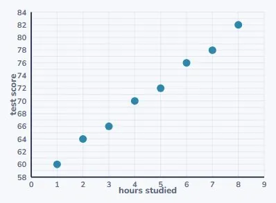
- Hours studied and test score, for eight students.
- Each student is one dot: their hours across, their score up.
- And the cloud clearly slopes upward.
Which variable goes on which axis
- The explanatory variable goes across the bottom.
- The response variable goes up the side.
- Ask: which of the two could plausibly affect the other?
| Axis | Variable | Here |
|---|---|---|
| x-axis | the explanatory variable | hours studied |
| y-axis | the response variable | test score |
| The test | which could affect the other? | |
| Study affects score | not the other way round |
That test works because the arrow only points one way
- Studying longer could change your score.
- Your score cannot reach back and change how long you studied.
- So hours is explanatory, and it goes on x.
| Hours | Score | Hours | Score |
|---|---|---|---|
| 1 hour | 60 | 5 hours | 72 |
| 2 hours | 64 | 6 hours | 76 |
| 3 hours | 66 | 7 hours | 78 |
| 4 hours | 70 | 8 hours | 82 |
The line of best fit is drawn by eye
- That is not a shortcut. It is the method at this level.
- Through the middle, with about as many points above as below.
- It will miss most of the points, and that is correct.
| Rule | ||
|---|---|---|
| Through the middle of the cloud | ||
| Roughly as many above as below | ||
| It will miss most of the points | that is correct | |
| Do not join the dots | that is a different, wrong thing |
And then you use it to predict
- What score might five and a half hours give?
- Up from 5.5 to the line, then across. About 74.
- Check it is sensible: between the 72 and the 76. It is.
| Step | Working | Note |
|---|---|---|
| Question | what score for 5.5 hours? | |
| Go up from 5.5 | to the line, then across | |
| Read off | about 74 | |
| Sensible? | between 72 and 76 | yes |
What to take away
- Six things, and the fourth one you will see in the news.
| A distribution | is the values and how often each occurred |
| The graph | is chosen by the kind of variable, not by taste |
| Every graph needs | the variable, the group, and the units |
| A y-axis not starting at zero | exaggerates the difference |
| The explanatory variable | goes on x, the response on y |
| A line of best fit | is drawn by eye and misses most points |
Your turn
- Pause here and try all four.
- Answers are in the description.
| Question | |
|---|---|
| 1 | Favourite sport per student. Which graph? |
| 2 | Sleep and reaction time. Graph? Which axis? |
| 3 | Bars of 100 and 105, axis from 95. Wrong? |
| 4 | Should a line of best fit pass through every point? |
Show answer
1. A bar graph. Favourite sport is one categorical variable. 2. A scatter plot, because they are two paired numerical variables. Hours slept goes on x, since sleep could affect reaction time, and reaction time goes on y. 3. The difference is only 5 percent, but starting at 95 makes the second bar look twice as tall. The numbers are honest and the picture is not. 4. No. It should pass through the middle of them, with roughly as many above as below, and it will miss nearly all of them. Joining the dots is a different thing and it is not a line of best fit.
The answers
- Favourite sport is one categorical variable.
- Sleep could affect reaction time, not the reverse.
- A line of best fit misses most points.
| Answer | |
|---|---|
| 1 | A bar graph |
| 2 | Scatter, sleep on x |
| 3 | The axis exaggerates |
| 4 | No |
Is your child on track?
Take the free placement test