A physics investigation with a non-linear relationship
What this lesson covers
- What Achieved, Merit and Excellence need in this internal, and what the evidence looks like.
- Planning: the independent, dependent and controlled variables, a sensible range, at least five values and repeats.
- Techniques that make measurements more accurate, and why each one works.
- Recognising a non-linear graph and choosing what to plot to make it straight: squares, square roots and inverses.
- Finding the gradient, writing the equation in the real variables, and discussing limits, difficulties, unexpected results and the physics.
What the standard asks for
- You carry out a practical investigation, usually given an aim and an outline method, and hand in your own results, graphs, conclusion and discussion; a template is not allowed.
- Each grade builds on the one before, and the marker judges the whole report, so the discussion counts as much as the data.
- The relationship must be non-linear, so the raw graph is a curve; you then plot a changed variable, such as a square or an inverse, to get a straight line.
| Grade | What you must show |
|---|---|
| Achieved | At least five values of the independent variable over a sensible range; a graph of the two variables; a conclusion naming the type of relationship |
| Merit | Control of a variable that really would change the results; techniques that improve accuracy, such as repeating and averaging; an equation with a gradient, written in the real variables |
| Excellence | A discussion of about two strong points: why the range has limits, why a control matters, how difficulties were overcome, the physics behind the result, or an unexpected result and its effect |
Planning the pendulum investigation
- Aim: find the relationship between the length of a pendulum and its period, the time for one complete swing, there and back.
- Independent variable: the length L, from the pivot to the centre of the bob, set at 0.20, 0.40, 0.60, 0.80, 1.00 and 1.20 m: six values over a range six times wide.
- Dependent variable: the period T, found by timing 10 complete swings and dividing by 10, three times for each length.
- Controlled variable that matters: the starting angle, kept at 10° with a protractor, because bigger swings take measurably longer.
- Also kept the same: the bob, the string and the clamp, so the only thing changing between runs is the length.
Techniques that make the timing accurate
- Time 10 swings, not one: your reaction time adds about the same error, perhaps 0.2 s, to any timing, which is 10% of a 2 s swing but only 1% of a 20 s run.
- Repeat each length three times and average: a random slip, early or late on the stopwatch, partly cancels out.
- Use a fiducial marker, such as a pointer or a strip of tape, at the lowest point of the swing, and start and stop the stopwatch as the bob passes it; the bob is moving fastest there, so the moment it passes is easiest to judge.
- Count "zero" as you start the stopwatch, so you do not stop one swing short.
- Measure the length to the centre of the bob with your eye level with the ruler, to avoid parallax error.
Example: the class's raw results
- A Year 12 class timed 10 swings three times at each length.
- Find the mean time for 10 swings at each length.
| Length (m) | Trial 1 | Trial 2 | Trial 3 | Mean |
|---|---|---|---|---|
| 0.20 | 8.9 | 9.1 | 9.0 | 9.0 |
| 0.40 | 12.6 | 12.8 | 12.7 | 12.7 |
| 0.60 | 15.4 | 15.7 | 15.4 | 15.5 |
| 0.80 | 18.1 | 17.9 | 18.0 | 18.0 |
| 1.00 | 20.1 | 19.8 | 20.1 | 20.0 |
| 1.20 | 22.0 | 22.1 | 21.9 | 22.0 |
- 0.20 m: (8.9 + 9.1 + 9.0) ÷ 3 = 27.0 ÷ 3 = 9.0 sadd the trials, divide by three
- 0.60 m: (15.4 + 15.7 + 15.4) ÷ 3 = 46.5 ÷ 3 = 15.5 s
- 1.00 m: (20.1 + 19.8 + 20.1) ÷ 3 = 60.0 ÷ 3 = 20.0 s
- the trials agree to within 0.3 s, about the size of a reaction time, so no result is left out
Spotting a non-linear relationship
- Plot the dependent variable (period) up the side and the independent variable (length) along the bottom, with units, and draw a smooth curve of best fit.
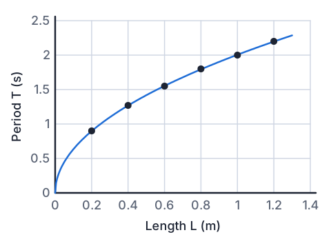
- The pendulum's curve starts at the origin and rises ever less steeply: a longer pendulum has a longer period, but doubling the length does not double the period.
- That shape, rising and flattening, suggests T ∝ √L, so T² ∝ L, and plotting T² against L should give a straight line.
- Match the shape to the change you make, then test it by plotting: if the new graph is a straight line through the origin, the guess was right.
| Raw graph of y against x | Likely relationship | Plot for a straight line |
|---|---|---|
| Curves upward, steeper and steeper | y ∝ x² | y against x² |
| Rises, then flattens | y ∝ √x | y against √x, or y² against x |
| Falls steeply, then levels off | y ∝ 1/x | y against 1/x |
| Falls even more steeply | y ∝ 1/x² | y against 1/x² |
Example: from mean times to T²
- Find the period T for each length, then T², keeping three significant figures.
| Length L (m) | Period T (s) | T² (s²) |
|---|---|---|
| 0.20 | 0.900 | 0.810 |
| 0.40 | 1.27 | 1.61 |
| 0.60 | 1.55 | 2.40 |
| 0.80 | 1.80 | 3.24 |
| 1.00 | 2.00 | 4.00 |
| 1.20 | 2.20 | 4.84 |
- T = mean time ÷ 10the mean was for 10 swings
- 0.40 m: T = 12.7 ÷ 10 = 1.27 s, T² = 1.27² = 1.6129 ≈ 1.61 s²
- 0.60 m: T = 15.5 ÷ 10 = 1.55 s, T² = 1.55² = 2.4025 ≈ 2.40 s²
- T² has units of s², and the column heading says so
Example: the straight-line graph and its equation
- Plot T² against L. The points lie close to a straight line through the origin, so T² is directly proportional to L.
- Find the gradient from a point that lies exactly on the line of best fit, far from the origin, not from a data point that is off the line.
- Write the equation in the real variables, with units.
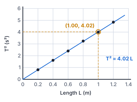
- the line passes through (0, 0) and (1.00 m, 4.02 s²)both points read off the line itself
- gradient = rise ÷ run = 4.02 s² ÷ 1.00 m = 4.02 s² m⁻¹
- T² = 4.02 L, with T in s and L in m
- taking the square root: T = 2.00√L, so the period is proportional to the square root of the length
Linking the result to the physics
- For small swings, physics predicts T = 2π√(L ÷ g), which squares to T² = (4π² ÷ g) × L.
- That is the same form as the class's T² = 4.02 L, so the gradient should equal 4π² ÷ g.
- Rearranging, g = 4π² ÷ gradient = 39.48 ÷ 4.02 = 9.82 m s⁻².
- That is within 0.2% of the 9.8 m s⁻² used in NCEA physics, which is strong evidence the measurements were accurate and the theory holds.
- The mass of the bob does not appear in the formula, which is why it was not the variable to control most carefully.
Excellence: writing the discussion
- Limits of the range: below 0.20 m, ten swings take under 9 s, so reaction time is a bigger share of each timing, and the bob's size makes its centre hard to measure to; above 1.20 m the bob began to swing in an ellipse, so it passed the marker at different points and the timing became less reliable.
- Why the control mattered: the formula only holds for small swings, and larger angles make the period measurably longer, so a changing angle would have added a second cause of changes in T.
- A difficulty overcome: at first the class lost count of swings, so they counted "zero" on release and timed from the marker, which also made each start sharper.
- An unexpected result: one 0.60 m trial (15.7 s) was 0.3 s above the other two, probably a late stop. It raises the mean by only 0.1 s and the point still sits on the line, so it does not change the conclusion.
- Had the line cut the L axis instead of passing through the origin, that would point to a systematic error, such as measuring to the top of the bob, not its centre.
Example: conclusions at each grade
- Achieved names the type of relationship; Merit gives the equation with the transformed variable; Excellence explains why it is so, and how far to trust it.
| Grade | What the student wrote |
|---|---|
| Achieved | As the length increases, the period increases, but not in a straight line. The graph of T² against L is a straight line through the origin, so T² is proportional to L. |
| Merit | T² is directly proportional to L. The gradient of the T² against L graph is 4.02 s² m⁻¹, so T² = 4.02 L. I kept the starting angle at 10° because a bigger swing takes longer. |
| Excellence | T² = 4.02 L matches the theory T² = (4π² ÷ g)L, giving g = 9.82 m s⁻², within 0.2% of 9.8 m s⁻². The small spread between trials (at most 0.3 s in runs of 9 to 22 s) shows that timing 10 swings and averaging kept reaction-time error small, so the conclusion is reliable over 0.20 to 1.20 m. |
Common mistakes
- The relationship is T² = 4.02 L, so I wrote y = 4.02x.Write the equation in the real variables with units: T² = 4.02 L, T in seconds and L in metres.
- I worked out the gradient from my first and last data points.Use points that lie exactly on the line of best fit, far apart, because data points off the line give a different gradient.
- I kept the mass of the bob the same, so that is my controlled variable.Mass has no effect on the period; for Merit, describe a control that would change the results, such as the starting angle.
- My graph of T against L is a curve, so there is no relationship.A smooth curve is a relationship; plot a transformed variable, such as T² against L, to make it straight.
A pendulum on the kitchen table
You need: a 1.5 m length of string, a bunch of keys or a large metal nut, strong tape, a tape measure, a phone stopwatch, paper and a pen
- Tie the keys firmly to the string and tape the other end to the edge of a high table or bench, so the keys hang freely.
- Set the length, from the tape to the middle of the keys, to 0.20 m, pull the keys about a hand's width to one side and let go.
- Time 10 complete swings, starting the stopwatch on "zero", and repeat twice more.
- Repeat for lengths of 0.40, 0.60, 0.80 and 1.00 m, then work out T and T² for each.
- Look for: T² divided by L comes out close to 4 every time, so T² is proportional to L, and a 1.00 m pendulum swings once every 2 seconds.
Safety: Swinging keys can fly off and hit an eye if the knot slips, so tie it tightly, check it before each run, and keep your face out of the swing's path.
Your turn
Theory says the height h a ball falls is proportional to t², where t is the time. What should you plot to get a straight line?
At a fixed voltage, current I is proportional to 1/R. What should you plot to get a straight line?
A pendulum's period is 1.40 s. Find T².
A graph of I against 1/R has a line of best fit through the origin and (0.10 Ω⁻¹, 0.60 A). Find the gradient and write the equation.
Explain why timing 10 swings gives a more accurate period than timing one.
Show answer
1. h against t². 2. I against 1/R. 3. T² = 1.40² = 1.96 s². 4. Gradient = 0.60 ÷ 0.10 = 6.0 A Ω (that is, 6.0 V), so I = 6.0 ÷ R. 5. The reaction-time error, about 0.2 s, is the same for any timing, so over 10 swings it is a ten times smaller share of the time, and dividing by 10 shrinks it in the period too.
Your turn: a marble on a ramp
- Another Year 12 class let a marble roll from rest down a ramp and measured the time t to roll each distance d, three times each.
- 1. Their graph of d against t curves upward, steeper and steeper. What should they plot to get a straight line?
- 2. Find t² for d = 0.40 m.
- 3. The straight-line graph has its line of best fit through the origin and (4.00 s², 1.00 m). Find the gradient and write the equation.
- 4. Name a controlled variable that would change the results if it changed, and say why.
| Distance d (m) | Mean time t (s) |
|---|---|
| 0.20 | 0.89 |
| 0.40 | 1.26 |
| 0.60 | 1.55 |
| 0.80 | 1.79 |
| 1.00 | 2.00 |
Show answer
1. d against t². 2. t² = 1.26² = 1.5876 ≈ 1.59 s². 3. Gradient = 1.00 m ÷ 4.00 s² = 0.25 m s⁻², so d = 0.25t². 4. The angle of the ramp: a steeper ramp gives the marble a bigger acceleration, so it would cover each distance faster.
Pendulum Lab
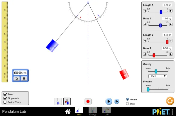
Full screen · PhET Interactive Simulations, University of Colorado Boulder, CC BY 4.0
Recap
- Plan six or more values over a wide range, with repeats, and control the variable that really affects the result.
- Time many swings, use a marker at the fastest point and average, and say why each technique helps.
- A curved raw graph is a clue: transform a variable until the graph is a straight line through the origin.
- Take the gradient from points on the line, and write the equation in the real variables with units.
- For Excellence, discuss the range limits, the controls, difficulties, unexpected results and the physics.
| If theory says | Plot | Gradient means |
|---|---|---|
| T = 2π√(L ÷ g) | T² against L | 4π² ÷ g |
| d = ½at² | d against t² | a ÷ 2 |
| I = V ÷ R | I against 1/R | V |
The maths behind it
How is NCEA Level 2 maths going?
See the NCEA Level 2 maths guide