PhysicsAS 91521NCEA Level 3 Science

Testing a physics theory by experiment

What this lesson covers

What the internal asks for at Achieved, Merit and Excellence, and how a theory with two variables is chosen and tested.
Planning: a wide range of the independent variable, controlled variables and techniques that make each reading more accurate.
Uncertainty in raw data from repeats and instrument readings, and how it carries through when a value is squared or divided.
Linearising a non-linear relationship so the graph is a straight line whose gradient means something physical.
Best-fit, steepest and shallowest lines, and a conclusion that compares the result with the theory quantitatively.

Key idea

How this internal works

Your teacher gives you a theory linking two variables in a curved (non-linear) way, such as a period and a mass, and you design and run the experiment yourself, usually over a few lessons, then write a report.
Achieved needs relevant data over a sensible range, uncertainties in the raw data, a graph you analyse to get an equation or a constant, and a conclusion that compares it with the theory.
Merit adds control of the variables that matter, techniques that improve accuracy, uncertainty carried onto the graph and into the gradient, and a comparison with numbers in it.
Excellence adds a discussion of the issues that could change your conclusion: variables that may have drifted, where the theory stops working, and anything unexpected in your results.

Key idea

Choosing a relationship to test

Pick a theory with one variable you can set accurately over a wide range (at least five or six values) and one you can measure many times.
Prefer relationships where the gradient or intercept gives a constant you can check another way, because that makes the comparison with theory easy to quantify.
This lesson follows a class testing a mass on a spring, where theory predicts T = 2π√(m/k) and k can also be found by simply hanging masses on the spring.

Theory	Vary	Measure	Straight-line graph
Mass on a spring: T = 2π√(m/k)	mass m	period T	T² against m, gradient 4π²/k
Pendulum: T = 2π√(L/g)	length L	period T	T² against L, gradient 4π²/g
String: f = (1/2L)√(F/μ)	tension F	frequency f	f against √F, gradient 1/(2L√μ)
Light intensity: I = P/(4πr²)	distance r	intensity I	I against 1/r²

Key idea

Method: control and accuracy

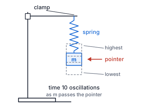
Hang the spring from a firm clamp stand and add slotted masses from 0.100 kg to 0.500 kg in 0.100 kg steps, checking each on an electronic balance.
Keep the amplitude small and the same each time (about 2 cm), pull straight down so the mass does not swing sideways, and use the same spring throughout so k stays fixed.
Fix a pointer level with the rest position and start and stop timing as the mass passes it, where it moves fastest, so the moment is easiest to judge.
Time 10 oscillations rather than one, so your reaction time of about 0.1 s is spread over ten periods, and repeat each timing three times.

A spring hanging from a clamp stand with a slotted mass on it, a pointer fixed level with the mass's rest position, and the mass shown at its highest and lowest points

Key idea

Uncertainty in the raw data

For repeated readings, the uncertainty is half the range: three times of 4.66 s, 4.86 s and 4.77 s give a mean of 4.76 s ± 0.10 s.
Dividing by a counted number keeps the percentage the same, so 10T = 4.76 ± 0.10 s gives T = 0.476 ± 0.010 s.
Squaring doubles the percentage uncertainty: 0.010 ÷ 0.476 is 2.1%, so T² = 0.227 s² ± 4.2%, which is ± 0.010 s².
For a single reading, use the instrument: half the smallest division for a scale, or the last digit for a digital balance, unless your technique (such as reaction time) is worse.

Key idea

Linearising the theory

A curve is hard to test by eye, so rearrange the theory into the form y = mx + c with the measured quantities on the axes.
Square T = 2π√(m/k) to get T² = (4π²/k) × m, so a graph of T² against m should be a straight line through the origin with gradient 4π²/k.
If you do not know the power, plot log T against log m: the gradient of a log-log graph is the power, so 0.5 here.
The straight line is the test: points that curve away from it, or an intercept far from zero, tell you something the theory leaves out.

Key idea

Try it: straighten a curve by squaring

Worked example

Example: one class's spring data

A Year 13 class timed 10 oscillations three times for each mass on one spring.
Process the 0.300 kg row into T and T² with uncertainties; the other rows were done the same way.

A Year 13 class's results for one spring
m (kg)	10T, three trials (s)	T (s)	T² (s²)
0.100	4.66, 4.86, 4.77	0.476 ± 0.010	0.227 ± 0.010
0.200	6.42, 6.60, 6.52	0.651 ± 0.009	0.424 ± 0.012
0.300	7.78, 7.98, 7.90	0.789 ± 0.010	0.623 ± 0.016
0.400	8.95, 9.14, 9.05	0.905 ± 0.010	0.819 ± 0.018
0.500	9.98, 10.18, 10.10	1.009 ± 0.010	1.018 ± 0.020

mean 10T = (7.78 + 7.98 + 7.90) ÷ 3 = 7.887 skeep the extra digit until the end
uncertainty = (7.98 − 7.78) ÷ 2 = 0.10 shalf the range of the repeats
T = 7.887 ÷ 10 = 0.789 s ± 0.010 sthe same 1.3% after dividing by 10
T² = 0.789² = 0.6225 s²; % uncertainty = 2 × 1.27% = 2.5%squaring doubles the percentage
T² = 0.623 ± 0.016 s²

Worked example

Example: gradient, intercept and their uncertainty

Plot T² against m with error bars, draw the best-fit line, then the steepest and shallowest lines that still pass through every error bar.
Find k from the gradient, with its uncertainty, and say what the intercept means.

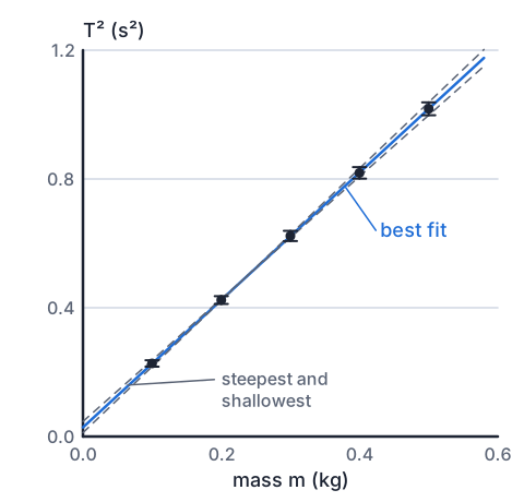
Graph of T² in s² against mass in kg: five points with error bars from 0.1 to 0.5 kg, a blue best-fit line and dashed steepest and shallowest lines through the ends of the error bars

best fit: gradient = 1.98 s² kg⁻¹, intercept = 0.029 s²least squares through the five points
steepest: (1.018 + 0.020 − (0.227 − 0.010)) ÷ (0.500 − 0.100) = 0.821 ÷ 0.400 = 2.05 s² kg⁻¹
shallowest: (1.018 − 0.020 − (0.227 + 0.010)) ÷ 0.400 = 0.761 ÷ 0.400 = 1.90 s² kg⁻¹
gradient = 1.98 ± 0.08 s² kg⁻¹half the spread of the extreme lines
k = 4π² ÷ 1.98 = 19.94 N m⁻¹; range 4π² ÷ 2.05 = 19.3 to 4π² ÷ 1.90 = 20.8gradient = 4π²/k
k = 20.0 ± 0.8 N m⁻¹

Key idea

Try it: fit a line to the class's data

Key idea

Comparing with the theory

The points lie on a straight line within their error bars, so T² is proportional to m (plus a small constant), which supports T = 2π√(m/k).
The class also hung 0.500 kg on the spring and measured a stretch of 0.243 m, so k = (0.500 × 9.81) ÷ 0.243 = 20.2 N m⁻¹, which lies inside 20.0 ± 0.8 N m⁻¹: the two methods agree.
The intercept is not zero: 0.029 s² ÷ 1.98 s² kg⁻¹ = 0.015 kg, as if 15 g extra were oscillating. The spring itself moves too, and theory for a real spring adds about one third of its own mass.
Write the conclusion as an equation with numbers: T² = (1.98 ± 0.08)m + 0.029, giving k = 20.0 ± 0.8 N m⁻¹, consistent with the static value.

Key idea

What lifts the report to Excellence

Discuss variables that could have changed and how: a spring warmed by handling, or stretched beyond its limit by the largest mass, would change k and bend the graph.
Discuss where the theory stops applying: it assumes a massless spring and a perfectly elastic one, so very small masses (comparable to the spring's mass) or very large stretches will not fit.
Explain anything unexpected and its effect on validity, such as the intercept: it does not invalidate the gradient, but a line forced through the origin would have given a wrong k.

Grade	A conclusion that reaches it
Achieved	T² against m is a straight line with gradient 1.98 s² kg⁻¹, so k = 20.0 N m⁻¹, close to the 20.2 N m⁻¹ found by stretching the spring.
Merit	The gradient is 1.98 ± 0.08 s² kg⁻¹, so k = 20.0 ± 0.8 N m⁻¹. The static value of 20.2 N m⁻¹ lies within this range, so the data support the theory.
Excellence	As Merit, plus: the 0.029 s² intercept matches about 15 g of extra moving mass, roughly a third of the 45 g spring, a mass the simple theory ignores. Because it shifts the line without changing the gradient, k is still valid.

Common mistakes

I timed one oscillation five times and averaged it, so my reaction time does not matter.
Time 10 or more oscillations each go, so the same reaction error is a tenth of the size per period.
T has a 1.3% uncertainty, so T² has a 1.3% uncertainty too.
Squaring doubles the percentage uncertainty, so T² has 2.6%.
The theory has no constant term, so I forced my best-fit line through the origin.
Draw the line the data give; an intercept is evidence you discuss, and forcing it changes the gradient.
My value of k is 20.0 and the other method gave 20.2, so they are different.
Compare using uncertainties: 20.2 lies inside 20.0 ± 0.8 N m⁻¹, so the values agree.

Try it at home

Find g with a string pendulum

You need: about 1.2 m of string, a bunch of keys or a small bag of rice, a door frame or hook, sticky tape, a phone stopwatch, a tape measure

Tie the keys to the string and tape the other end to the top of a door frame so the keys hang freely.
Set the length from the top to the middle of the keys to 1.00 m, pull the keys about 5 cm to one side and time 10 swings, three times.
Repeat for lengths of 0.80, 0.60, 0.40 and 0.20 m, and work out T and T² for each.
Plot T² against L and find g = 4π² ÷ gradient.
Look for: a straight line through close to the origin and a value of g near 9.8 m s⁻²; big swings will push your T values up.

Safety: Keep the swing small and the area clear, because heavy keys swinging at head height can hit someone walking through the doorway.

Your turn

Three timings of 10 oscillations are 8.42 s, 8.50 s and 8.46 s. Find T with its uncertainty.

Using T = 0.846 ± 0.004 s, find T² with its absolute uncertainty.

Theory says f = (1/2L)√(F/μ), with tension F varied. What should you plot to get a straight line?

A graph of T² against m has gradient 2.47 s² kg⁻¹. Find the spring constant k.

The steepest and shallowest lines on a graph have gradients 2.55 and 2.40 s² kg⁻¹. What is the uncertainty in the gradient?

Show answer

1. Mean 10T = (8.42 + 8.50 + 8.46) ÷ 3 = 8.46 s, uncertainty (8.50 − 8.42) ÷ 2 = 0.04 s, so T = 0.846 ± 0.004 s. 2. T² = 0.846² = 0.716 s²; percentage uncertainty 2 × (0.004 ÷ 0.846) = 0.95%, so T² = 0.716 ± 0.007 s². 3. f against √F, a straight line through the origin with gradient 1/(2L√μ). 4. gradient = 4π²/k, so k = 4π² ÷ 2.47 = 39.48 ÷ 2.47 = 16.0 N m⁻¹. 5. (2.55 − 2.40) ÷ 2 = ± 0.08 s² kg⁻¹ (0.075 rounded).

Try it

Pendulum Lab

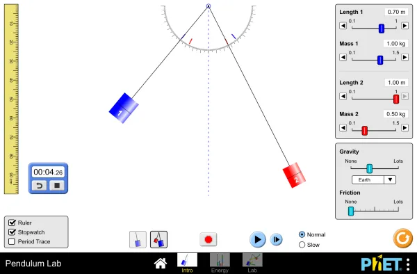
Full screen · PhET Interactive Simulations, University of Colorado Boulder, CC BY 4.0

Summary

Recap

Choose a theory you can test over at least five or six values, ideally with a constant you can check another way.
Control the other variables and use techniques such as timing many oscillations and a fiducial marker.
Uncertainty: half the range of repeats; percentages stay the same when dividing by a count and double when squaring.
Linearise, plot with error bars, and get the gradient's uncertainty from the steepest and shallowest lines.
Conclude with an equation, a constant with its uncertainty, a comparison with theory, and a discussion of what could change it.

Step	In the spring example
Theory	T = 2π√(m/k)
Linear form	T² = (4π²/k)m
Gradient	1.98 ± 0.08 s² kg⁻¹
Result	k = 20.0 ± 0.8 N m⁻¹
Check	static k = 20.2 N m⁻¹, inside the range

Maths

The maths behind it

Year 13 MathsFitting a linear model

Report a mistake

How is NCEA Level 3 maths going?

See the NCEA Level 3 maths guide